Exploring the Goodness-of-Fit Test in R

Background

One of the common statistical tests is the goodness-of-fit (GOF) test, which is simply used to test whether the observed data fit into a particular theoretical distribution (i.e. normal, log-normal, poisson, expotenial, binormial, uniform, etc.). Selecting the preferrable distribution for the particular uncertain parameters is essential in probability such as Monte Carlo sampling. Several well-known statistical tests used to validate the GOF are Chi-square test, Anderson-Darling, Kolmogorov-Smirnov test, and Cramer-Von Mises creterion. In this post, we will explore the GOF test in R using the fitdistrplus package. All essential tests mentioned above can be called in fitdistrplus. The package is available in CRAN and can be installed using the following command:

$install.packages("fitdistrplus")  

library(fitdistrplus)

Null Hypothesis

To interpret the GOF test, we need to define the null hypothesis statement. Null hypothesis is a hypothesis that is assumed to be true unless proven otherwise, and p-values are used to test the null hypothesis. Simply, p-values are numbers between 0 and 1 to quantify how confident the sample data is different from a theoretical distribution. The closer a p-value is to 0, the more confidence we can state that the sample data set and theoretical distribution is different. The question is how small does a p-value have to be before we are sufficiently confident that the sample data is different from theoretical distribution. Hence, there is a need to set a threshold value for the p-value to reject the null hypothesis. The threshold value is called the statistical significance level, denoted as $`\alpha`$, and it is practically set to 0.05. If the p-value is less than $`\alpha`$, we reject the null hypothesis. Otherwise, we accept the null hypothesis.

With the above explanation, the null hypothesis statement of the GOF test is defined as follows 😦 😎:
Definition:

Null Hypothesis : The sample data is generated from a theoretical distribution
Alternative hypothesis : The sample data is not generated from a theoretical distribution
$\alpha = 0.05$

Inference:

p-value < 0.05: Reject the null hypothesis - The sample data is not generated from a theoretical distribution
p-value > 0.05: Accept the null hypothesis - The sample data is generated from a theoretical distribution

Goodness-of-Fit Test in R

Once installing the fitdistrplus and setting the null hythothesis statement, we will explore the GOF test in R by both graphical and statistical methods. The following code is used to define the function gof_fit:

gof_fit <- function(data, dist_type, test_type){ 

  # dist_type can be 'norm','lnorm','pois','exp','gamma','bninom','geom','beta','unif','logis'
  # test_type: sw (Shapiro-Wilk), ad, cmv, lillie, skew, chisq, ks

  fit_func <- fitdist(data, dist_type)
  gof = gofTest(data,distribution = dist_type, test = test_type)
  
  plot(fit_func)
  print(gof)
}

📝 Note:
The function fitdist takes two arguments: data is the sample data, and dist_type is the distribution to be tested.
The gofTest function takes three arguments: data is the sample data, distribution is the distribution to be tested, and test is the statistical test to be used. The following code is used to define the function, in addition to plotting the histogram and density plot and printing the GOF test results:

In the following sections, we will utilize the defined function to investigate the GOF for two data sets. The first data set is generated from a pre-defined normal distribution. We will explore the fundamental concept as mentioned in the previous sections. Subsequently, we will practice with actual oil and gas data set.

Sample Data

The sample data is generated using the rnorm function in R. The rnorm function is used to generate random numbers from a normal distribution. The rnorm function takes three arguments: n is the number of random numbers to be generated, mean is the mean of the normal distribution, and sd is the standard deviation of the normal distribution. The following code is used to generate the sample data with mean 0 and standard deviation 1:

set.seed(123)
x <- rnorm(10000, mean = 0, sd = 1)

Let’s run the gof_fit function to test the GOF for the normal distribution and the chi-square test:

x_gof <- gof_fit(x, "norm", "chisq")

Sample data and theoretical data can be displayed in the same graph:

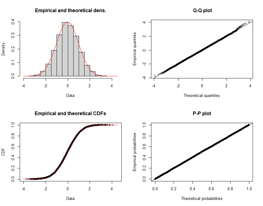
GOF test results are printed out as follows:

Results of Goodness-of-Fit Test
-------------------------------

Test Method:                     Chi-square GOF

Hypothesized Distribution:       Normal

Estimated Parameter(s):          mean = -0.02640343
                                 sd   =  1.00017354

Estimation Method:               mvue

Data:                            df_normal

Sample Size:                     10000

Test Statistic:                  Chi-square = 86.832

Test Statistic Parameter:        df = 77

P-value:                         0.2078002

Alternative Hypothesis:          True cdf does not equal the
                                 Normal Distribution.

📝 As the p-value = 0.207, which is greater than 0.05, we accept the null hypothesis and conclude that the sample data is generated from a normal distribution.

Actual Hydrocarbon Data

In the following works, we will use examine the GOF with actual hydrocarbon data. This data set contains 189 data points; each data point represents the total hydrocarbon thickness of a particular oil & gas field. The data is stored in a csv file and can be loaded using the read.csv function in R. The following code is used to load the data and genrate the descriptive statistics:

df <- read.csv("data.csv")
desdist(df, boot = 1000)

summary statistics
------
min:  8   
max:  410 
median:  125 
mean:  141.7063 
estimated sd:  88.94661 
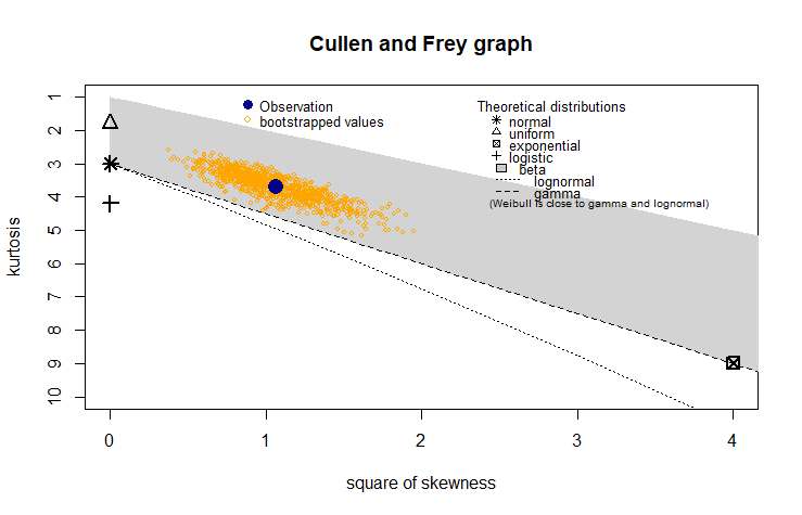
estimated skewness:  1.031698 
estimated kurtosis:  3.684621

Skewness and Kurtosis are used to measure the asymmetry and the peakedness of the distribution. The skewness and kurtosis of the sample data are 1.03 and 3.68, respectively; inferring that the sample data is slightly skewed and peaked, which is not normal distribution and right-skewed distributions could be considered such as lognormal, gamma, and Weibull. Additionally, a skewness-kurtosis plot such as one proposed by Cullen and Frey (1999) as shown in the following figure can be used to visually check the distribution type. However, skewness and kurtois are known not to be reliable for small sample sizes, therefore a bootstrapping method by random sampling is used to estimate the skewness and kurtosis.

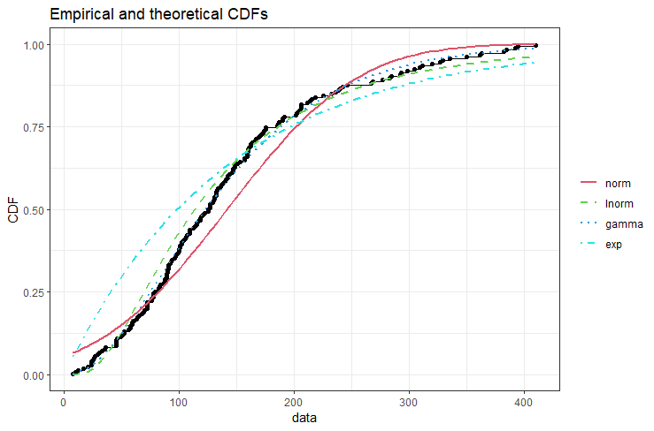
Herein, we will use the cdfcomp function to compare the sample data with several theoretical distributions using cummulative density plot.

fit_norm <-fitdist(df_pay,"norm")
fit_logn <-fitdist(df_pay,"lnorm")
fit_gama <-fitdist(df_pay, "gamma")
fit_exp  <-fitdist(df_pay, "exp")

cdfcomp(list(fit_norm, fit_logn, fit_gama, fit_exp),plotstyle = "ggplot")

GOF test results for lognormal with Kolmogorov-Smirnov test:

Results of Goodness-of-Fit Test
-------------------------------

Test Method:                     Kolmogorov-Smirnov GOF

Hypothesized Distribution:       Lognormal

Estimated Parameter(s):          meanlog = 4.7330949
                                 sdlog   = 0.7276173

Estimation Method:               mvue

Data:                            df

Sample Size:                     189

Test Statistic:                  ks = 0.08218303

Test Statistic Parameter:        n = 189

P-value:                         0.1556172

Alternative Hypothesis:          True cdf does not equal the
                                 Lognormal Distribution.

📝 As the p-value = 0.1556, which is greater than 0.05, we accept the null hypothesis and conclude that the sample data is fitted with a lognormal distribution.

The table below summarizes the GOF test results for the four distributions using Chi-square test:

Distribution Type	p-value	Result (Accept / Reject)	Inference
Normal	5.33e-06	Reject the Null Hypothesis	Alternative
LogNormal	0.1846	Accept the Null Hypothesis	Data is generated from this distribution type
Gamma	0.6037	Accept the Null Hypothesis	Data is generated from this distribution type
Expotenial	1.368e-08	Reject the Null Hypothesis	Alternative

💡 Conclusion: As the p-values of Lognormal and Gamma distributions in the table above are 0.1846 and 0.6037, respectively, which are greater than 0.05. Therefore, we accept the null hypothesis and conclude that the sample data is fitted in both lognormal distribution or gamma distribution.

---

😉 Today’s Quote: If you choose not to decide, you still have made a choice. - Neil Peart